What a technical indicator actually is
Open any chart and you see lines layered above and below the candles. Those are technical indicators — second-order values computed from price and volume.
There is only one source dataset. Each bar carries an open, high, low, close and volume, together called OHLCV. Every indicator comes out of that. None of them add information; they turn properties the eye cannot read off candles into numbers.
There are roughly four such properties: whether price has run too far in either direction (overheating), whether direction is turning (trend reversal), how violently it is moving (volatility), and which way the larger flow runs (long-term trend). Hundreds of indicators exist, but most are different ways of measuring one of those four.
So you do not need dozens to start. Cover each of the four once.
An agent calls exactly five
Take a concrete reference. Vibe-Trading, the open-source trading agent published by HKUDS (the Data Intelligence Lab at the University of Hong Kong), takes a natural-language instruction, fetches data and runs a backtest. Open the repository and the indicators the agent can call immediately through one tool number exactly five.
They sit as constants in agent/src/tools/technical_indicator_tool.py: RSI at 14, MACD at 12/26/9, Bollinger Bands at 20 bars with two standard deviations, SMA at 20/50/200, EMA at 20. The numbers in parentheses are window lengths — how many bars the calculation looks back over.
Those five map onto the four properties. RSI takes overheating, MACD takes reversal, Bollinger Bands take volatility, SMA and EMA take trend. The chart UI adds KDJ(9), but the agent-facing tool does not include it.
Why only five? Because everything derives from the same OHLCV, so indicators overlap heavily. Stochastics and RSI measure substantially the same thing; stacking both raises confidence without raising information. Stopping at five reads as a choice, not a gap.
| Indicator | Default parameters | What it measures | Range |
|---|---|---|---|
| RSI | 14 | Overbought / oversold | 0 – 100 |
| MACD | 12 / 26 / 9 | Timing of trend reversal | Price units (unbounded) |
| Bollinger Bands | 20, 2σ | Volatility corridor | Price units (upper/mid/lower) |
| SMA | 20 / 50 / 200 | Trend line | Price units |
| EMA | 20 | Recency-weighted trend line | Price units |
RSI(14) — scoring overheating from 0 to 100
RSI stands for Relative Strength Index. It weighs the force of up days against down days over the last 14 bars and collapses both into a single number.
Four steps. First, take the day-over-day change. Second, split it into gains on up days and losses on down days. Third, average each over 14 bars. Fourth, divide average gain by average loss to get RS and plug it into RSI = 100 - 100 / (1 + RS).
The shape of that formula pins the value between 0 and 100. Fourteen straight up days give an average loss of zero and an RSI of 100; the reverse gives 0. In practice it mostly oscillates between 30 and 70.
Reading it is convention. Above 70 is called overbought, below 30 oversold. Those two numbers do not fall out of the formula — J. Welles Wilder set them — so they are routinely adjusted per instrument and market.
One trap. In a strong uptrend RSI can sit above 70 for weeks. A rule that sells the moment it crosses 70 misses the whole opening leg of a rally. RSI reports strength, not direction, so it belongs next to a trend indicator.
MACD(12/26/9) — reversal as the distance between two averages
MACD is Moving Average Convergence Divergence. Long name, simple job: it measures the distance between a fast average and a slow one.
It produces three values. The MACD line is the 12-day EMA minus the 26-day EMA — positive when the short average sits above the long one, negative when below. The signal line smooths that MACD line with a 9-day EMA. The histogram is the MACD line minus the signal line, drawn as bars so the gap between the two is visible.
You read the crossings. When the MACD line crosses above the signal line, that is a golden cross and reads bullish; crossing below is a death cross. The histogram approaches zero slightly before the crossing, which is what makes it useful as an early tell.
The MACD line crossing zero is read separately. Passing above zero means the 12-day average has overtaken the 26-day one — the trend itself has flipped.
The trap is lag. Moving averages are averages of prices that already happened, so they react after the turn. On volatile assets signals arrive late, and in sideways ranges crossings repeat meaninglessly. Shortening the windows speeds it up and adds noise in equal measure.
Bollinger Bands(20, 2σ) — drawing a corridor out of volatility
Bollinger Bands are three lines. The middle is a 20-day simple moving average; the upper adds two 20-day standard deviations to it and the lower subtracts them. Price appears to travel through the corridor between.
The point is that the corridor is not a fixed width. Standard deviation is the size of volatility, so the bands widen when price swings hard and tighten when it goes quiet. What this indicator really shows is volatility, not position.
Hence the squeeze, the setup most traders actually watch for. When band width narrows unusually against recent history, volatility has died — and a large move in one direction usually follows. It forecasts magnitude, not direction.
The choice of two standard deviations has a rationale. If values were normally distributed, roughly 95% would fall within mean ± 2σ. Real price changes are not normal — the tails are fatter — so excursions outside the bands happen far more often than the theory implies.
Which means touching a band is not a signal. Selling every tag of the upper band keeps being wrong in a strong rally; riding the upper band has its own name, the band walk. Bands are better used to judge the volatility regime than the price level.
SMA(20/50/200) and EMA(20) — the oldest and most used trend lines
SMA is the simple moving average: add the last N closes and divide by N. The 20-day line is about a month, the 50-day about a quarter, the 200-day roughly a year of trading days.
The 200-day line gets special treatment for reasons of convention, not mathematics. Enough institutions use it as their long-term reference that whether price sits above or below it influences participant behaviour on its own.
EMA is the exponential moving average. Where SMA gives all 20 days equal weight, EMA weights recent prices more, with older prices decaying exponentially. It turns faster than SMA — and reacts to noise just as fast.
Overlaying two of them gives the golden and death crosses. A shorter average crossing above a longer one is a golden cross, crossing below a death cross. The common pairing is the 50-day against the 200-day.
The trap is the same as MACD's. Averages are backward-looking and therefore late. Golden crosses often print well after a rally is under way, and in a range the two lines tangle and flip signals repeatedly.
Computing all five yourself in pandas
You do not need a separate library — pandas alone produces all five. The only input is a close series, and all five functions fit in under ten lines each.
Save the code below as indicators.py and pass it a close-price pandas Series. Get the closes from yfinance, pykrx, or a broker CSV read with pandas.
adjust=False on ewm matters. The default True uses a different formula that corrects the initial window, so omitting it leaves the first few dozen bars of your EMA out of step with every other tool.
Once the functions exist, check them once. Pull the same ticker up in a broker app or on TradingView and compare RSI on the same date. The numbers may not match — which is what the next section is about.
import pandas as pd


def rsi(close: pd.Series, period: int = 14) -> pd.Series:
    delta = close.diff()
    gain = delta.clip(lower=0)
    loss = (-delta).clip(lower=0)
    avg_gain = gain.ewm(alpha=1 / period, adjust=False).mean()
    avg_loss = loss.ewm(alpha=1 / period, adjust=False).mean()
    return 100 - 100 / (1 + avg_gain / avg_loss)


def macd(close, fast=12, slow=26, signal=9):
    line = (close.ewm(span=fast, adjust=False).mean()
            - close.ewm(span=slow, adjust=False).mean())
    sig = line.ewm(span=signal, adjust=False).mean()
    return pd.DataFrame({"macd": line, "signal": sig, "hist": line - sig})


def bollinger(close, period=20, num_std=2.0, ddof=0):
    mid = close.rolling(period).mean()
    sd = close.rolling(period).std(ddof=ddof)
    return pd.DataFrame({"upper": mid + num_std * sd,
                         "middle": mid,
                         "lower": mid - num_std * sd})


def sma(close, period):
    return close.rolling(period).mean()


def ema(close, period):
return close.ewm(span=period, adjust=False).mean()import yfinance as yf
from indicators import rsi, macd, bollinger, sma, ema
close = yf.download("AAPL", period="1y")["Close"].squeeze()
print("RSI(14) :", round(rsi(close).iloc[-1], 2))
print("MACD :", macd(close).iloc[-1].round(4).to_dict())
print("BB(20,2):", bollinger(close).iloc[-1].round(2).to_dict())
print("SMA200 :", round(sma(close, 200).iloc[-1], 2))
print("EMA20 :", round(ema(close, 20).iloc[-1], 2))The same name is not the same number — two ways to smooth RSI
This is the part that matters most. Two tools can both say RSI 14 and report different values, because step three — averaging the gains and losses — comes in two flavours.
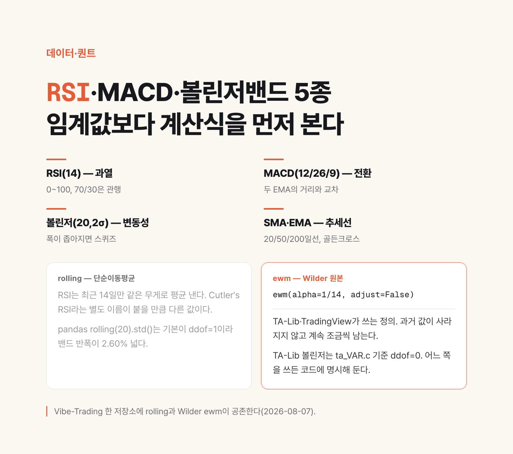
One is Wilder's method, the original: an exponentially weighted average with alpha = 1 / 14. Old values never fully drop out; they keep contributing a little. TA-Lib does it this way — its ta_RSI.c comments the step as "Wilder's approach" and multiplies the previous average by period-1, adds today's value and divides by period (source checked 2026-08-07).
The other is a plain simple moving average: weight the last 14 bars equally and discard the fifteenth. It is distinct enough to carry its own name, Cutler's RSI. It swings more sharply than Wilder's, and it can jump when a large value falls out of the window.
This is not hypothetical. In the Vibe-Trading repository, the RSI function in technical_indicator_tool.py computes with rolling(14).mean(). Yet the strategy skill in the same repository, technical-basic/SKILL.md, states explicitly that RSI and ADX use Wilder EWM — ewm(alpha=1/period). Both live in one repository (source checked 2026-08-07).
Neither is wrong; both are definitions in real use. The problem is backtesting on one and trading on the other without knowing. Same rule, different entry points. If your condition is RSI crossing 70, then 69.4 versus 71.2 is a different trade.
wilder = gain.ewm(alpha=1 / 14, adjust=False).mean()   # Wilder 원본 · TA-Lib ta_RSI.c
cutler = gain.rolling(14).mean()                       # Cutler's RSI · simple moving average

# build both RSIs from the same closes and compare the last value
print(round(rsi_wilder(close).iloc[-1], 2),
      round(rsi_cutler(close).iloc[-1], 2))
Bollinger has the same split — the ddof of the standard deviation
When you compute a standard deviation, what you divide the sum of squared deviations by comes in two flavours. Divide by n and you get the population standard deviation (ddof=0); divide by n - 1 and you get the sample one (ddof=1). Statistics conventionally uses n - 1 when estimating a population from a sample.
pandas rolling(20).std() defaults to ddof=1. Pass no arguments and you get the sample standard deviation.
TA-Lib does not. In its source, ta_BBANDS.c routes band width down to the variance in ta_VAR.c, and that formula is variance = sum(x²)/n - mean². Dividing by n makes it the population variance, hence ddof=0 (source checked 2026-08-07).
The gap is calculable. The sample standard deviation equals the population one times sqrt(n / (n - 1)). With n at 20 that is sqrt(20 / 19) = 1.0260, so bands drawn with the pandas default are 2.60% wider at the half-width than TA-Lib's.
2.60% sounds small until a band touch is your trading condition. On days when price sits near a band, one implementation fires and the other does not. That is why it is worth checking here before suspecting the strategy when a backtest does not match live trading.
The fix is trivial. Either convention is fine as long as backtest and live agree, so state ddof explicitly in code. That is what the ddof=0 default in the bollinger function above is for.
sd_sample = close.rolling(20).std()          # pandas default · ddof=1
sd_pop = close.rolling(20).std(ddof=0)       # population, matching TA-Lib

print(round(sd_sample.iloc[-1] / sd_pop.iloc[-1], 4))   # 1.026 = sqrt(20 / 19)
A checklist before you wire an indicator in
One, state the window length. RSI 14, MACD 12/26/9, Bollinger 20 are defaults and vary by tool. Writing them as arguments narrows the search when numbers stop matching.
Two, check the smoothing. Indicators Wilder created — RSI, ADX — define ewm(alpha=1/period) as the original. Whatever the library docs say, read the source and see whether it is rolling or ewm. It takes a minute.
Three, state ddof. This applies to every indicator built on a standard deviation, not just Bollinger Bands, including volatility used as a signal in its own right.
Four, check adjust on your EMA. The pandas ewm default adjust=True computes the initial window differently. Match other tools with adjust=False.
Five, do not build a trading rule on a single indicator. The technical-basic skill in Vibe-Trading computes three axes — trend (EMA and ADX), mean reversion (Bollinger Bands and RSI), and volume (OBV and volume ratio) — and votes them into one signal, entering only when all three agree and standing aside when they conflict.
In short: half of learning indicators is knowing what each one measures. The other half is knowing how your tool computes it. Skip the second half and you get numbers without knowing what they mean.