What a backtest is
A backtest applies your trading rule to past prices. You decide in advance when to buy and when to sell, step through the past months or years one day at a time, and calculate what your balance would be if you had traded that way. It is how you check whether a rule makes sense before real money is involved.
It is worth doing because most rules built on intuition fall apart in front of numbers. A rule that sounds reasonable in your head turns out to signal too late, or too often, or to move exactly the wrong way in the stretch that mattered. A backtest tells you that before you pay for the lesson.
At the same time a backtest is not a device for predicting the future. That something worked in the past guarantees nothing. What a backtest genuinely filters out is the clearly bad rule; what remains is a rule that was not bad. Miss this distinction at the start and you will lean on the numbers far more than they deserve.
This used to mean sourcing price data, arranging it into a table, and writing the loop yourself. Now two pieces suffice: an API that serves prices, and an AI agent that writes and runs code on your machine.
Start with data — daily OHLC from the candle endpoint
One term first. A candle compresses a day (or a minute) of price movement into four numbers: open, high, low and close, or OHLC. One candle per day is a daily candle, and a series of them is the minimum raw material a backtest needs.
The Toss Securities Open API serves this through its candle endpoint. The access token from the previous post is enough; no account header is required, because quotes are objective data served identically to every user.
Two things bite in practice. First, a single call returns at most 200 candles. A year of daily bars is roughly 250, so you have to feed the cursor that comes back with the response and walk further into the past. Second, request adjusted prices. For a stock that paid dividends or split, raw prices make the split day look like a crash, and the backtest reads it as one.
Sort what you collect in ascending date order and collapse duplicate dates into one. Stitching pages together tends to repeat a day at the boundary, and leaving it in counts that day twice, quietly inflating the return.
TOKEN=eyJ...

curl -s 'https://openapi.tossinvest.com/api/v1/candles?symbol=KORU&interval=1d&count=200&adjusted=true' \
  -H "Authorization: Bearer $TOKEN"

# response (excerpt)
# {"result":{
#   "candles":[{"timestamp":"2026-07-27T00:00:00",
#               "openPrice":18.02,"highPrice":18.9,
#               "lowPrice":17.71,"closePrice":18.45,"volume":...}],
# "nextBefore":"..."}}import os, requests
BASE = "https://openapi.tossinvest.com/api/v1/candles"
H = {"Authorization": f"Bearer {os.environ['TOSS_TOKEN']}"}
def daily_ohlc(symbol, need=400):
rows, before = {}, None
while len(rows) < need:
p = {"symbol": symbol, "interval": "1d",
"count": 200, "adjusted": "true"}
if before:
p["before"] = before
r = requests.get(BASE, params=p, headers=H, timeout=10).json()["result"]
if not r.get("candles"):
break
for c in r["candles"]: # date key removes duplicates
d = c["timestamp"][:10]
rows[d] = {"d": d, "o": float(c["openPrice"]),
"h": float(c["highPrice"]), "l": float(c["lowPrice"]),
"c": float(c["closePrice"])}
before = r.get("nextBefore")
if not before:
break
return [rows[d] for d in sorted(rows)] # oldest to newestFour things to pin down when you hand a rule to an agent
This is the heart of it. Describe a rule and the script arrives in minutes. The problem is that a rule stated in a sentence always leaves blanks, and the agent does not ask about them. It fills them quietly with whatever looks most plausible, then hands you a very convincing table of returns.
There are usually four blanks. Write these down alongside the rule and the spread of possible results narrows sharply.
First, the evaluation moment. When during the day is the condition checked? Checking on the close versus firing the instant an intraday price touches the level are two different strategies. Evaluate buy signals intraday and you will also buy every false breakout that had already collapsed by the close.
Second, the fill price. Once the condition is met, at what price are you deemed to have traded? The close, the level itself, the next day's open? As we will see, this single line moves the result more than anything else.
Third, trading costs. Decide what round-trip percentage covers commission, tax and spread. Leave it at zero and any strategy that trades often will look far better than it is.
Fourth, the data window. Which period are you using? Moving the start date alone frequently reverses the ranking. Winning in one window is not yet a conclusion.
| Item | If you leave it unstated | State it like this |
|---|---|---|
| Evaluation moment | Intraday signals slip in, including trades you could never have made | Buy conditions evaluate on the close only; ignore intraday touches |
| Fill price | The most favourable price gets assumed and returns inflate | Exits fill at the level; on a gap, fill at that day's open |
| Trading costs | Costs count as zero and frequent-trading strategies are overrated | Deduct 0.05 percent per side, 0.1 percent round trip, per trade |
| Data window | The best-looking period gets picked and the conclusion flips | Print the last 1 year, 3 years and full history separately |
Write a Python script that backtests the following rule on this candle data.

[Rule]
- Start fully invested at the start of the window
- While holding, sell everything on a 20% drop from the high
  (the high updates on intraday highs)
- While flat, buy everything when the close breaks the prior 20-day high
- While holding, sell everything when RSI(14, Wilder) exceeds 80

[Assumptions - use exactly these]
- Buy and RSI conditions evaluate on the close; the trailing exit
  evaluates on an intraday touch
- Trailing fill = high x 0.8; if the open gaps below that, fill at the open
- Deduct 0.1% round-trip cost on every trade
- Print the last 1 year / 3 years / full history separately

[Output]
- Trade log (date, side, fill price, reason)
- Return, max drawdown and buy-and-hold comparison per window
Why the same rule returned 15 percent and 95 percent
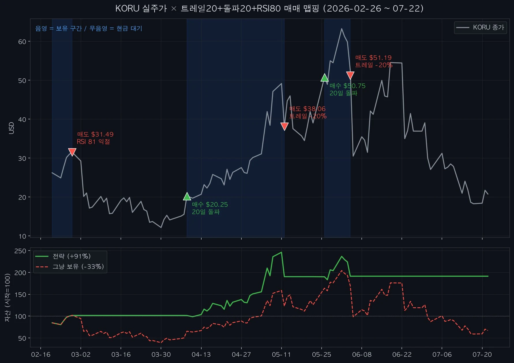
Stated abstractly this does not land, so I ran it. The subject is KORU, a US-listed ETF tracking the Korean market at 3x. The rule is exactly the one above: sell everything on a 20 percent drop from the high, buy everything when the close breaks a 20-day high, take profit when RSI passes 80. The window runs from 26 February to 22 July 2026, about five months.
Same rule, same candles, run twice. One thing changed: the exit fill. The first run assumed the sale happened at the closing price of the day the condition was met. The second assumed it happened at the level itself, the moment price touched it.
Close fills returned 15 percent. Touch fills returned 95 percent. Simply holding over the same period returned minus 33 percent. Not a character of the rule changed, and the results sit eighty points apart.
The gap came from a single day. After topping out in early June the fund halved within days. Filling at the level means leaving near 49 dollars; waiting for that day's close means leaving at 30. Because it is a 3x product the daily move is large, and that one assumption dominated the entire result.
Which is correct depends on how your system actually runs. A conditional order resting on the broker's server fires the moment price reaches the watch level, which is close to a touch fill. Judging by hand once a day on the close and ordering the next morning is worse than a close fill. So this is not a matter of taste; it is a value you copy from how you actually operate.
And either way, real fills are worse. In a fast decline you cannot sell everything at the price you wanted, and a market order slips further as the spread widens. That is why a backtest number should never be read as expected return.
# A. Close fill - check on the close, assume the sale at that close
if close[i] <= high * 0.8:
    fill = close[i]

# B. Touch fill - if the intraday low reaches the level, assume the level
level = high * 0.8
if low[i] <= level:
    fill = min(level, open[i])   # gap below? fill at the open

# same rule, same data, 2026-02-26 to 07-22
# A -> +15%   B -> +95%   buy and hold -> -33%
The variants actually tested on KORU
Once the assumptions are fixed, the real experiments begin: one change at a time on the same skeleton. On a 3x leveraged ETF the variants sorted out roughly as follows.
The most frequent idea was to make re-entry easier, because waiting for a 20-day high felt too slow. So I shortened the window to 10 days, discounted the threshold so it would buy slightly short of a new high, and swapped in rebound signals such as RSI 30 or moving-average crosses. Every one of these attempts underperformed the original.
Only two changes improved it: lengthening the window to 30 days, and taking profit while RSI is above 80 instead of waiting for the trailing exit. In other words the edge came not from a clever entry signal but from the patience to wait until a new high is confirmed.
I also tested splitting the position into pockets with different trailing percentages. Selling one half at 15 percent and the other at 20 percent looked like it would soften the drawdown, and it did not. Being the same instrument, both halves take the same crash and only the exit dates differ by a few days, so maximum drawdown barely moved while returns fell by however much the weaker parameter was mixed in. Splitting an asset with a correlation of one is not diversification.
Porting a logic that worked elsewhere also failed. A z-score ensemble used for minute-level crypto trading generated thousands of trades once laid over daily ETF bars. At zero cost it looked plausible; at 0.05 percent per side it collapsed. The logic was not bad, the time scale and cost structure simply did not match.
One more. The 200-day moving average filter that worked best on the 2x product was actively harmful on the 3x. With higher volatility it churned around the average and accumulated losses. Even within the same family, a different multiple wants a different filter.
| Change | Intent | Result |
|---|---|---|
| Re-entry window 20 to 10 days | Re-enter sooner | Sharply worse |
| Threshold discounted 10 percent | Buy just before the new high | Monotonically worse |
| Rebound-signal re-entry (10 kinds) | Catch the bottom | All worse |
| Re-entry window 20 to 30 days | Confirm for longer | Improved |
| Add RSI 80 profit take | Exit near the top | Improved |
| Split trailing rates (15+20, 20+25) | Soften drawdown | Worse in all three windows |
| Port minute-level z-score ensemble | Reuse logic from another market | Collapses once costs apply |
| 200-day moving average filter | Exit on trend break | Best on 2x, unsuitable on 3x |
Five places a backtest quietly lies
These are the first places to suspect when results look good. None of them raise an error; they simply return a nice number, so you have to go looking.
First, the fill assumption we just saw. Assuming an exact sale at the level flatters any strategy in a crash. Add a little slippage, run it again, and see whether the conclusion survives.
Second, leaked future information. If a value that requires knowing today's close drives a trade placed during today's session, trades that were never possible are contributing to the result. Including the current bar in an indicator calculation is the common way this happens.
Third, zero cost. Look at the trade count first, multiply by the round-trip cost, and check whether anything is left. If not, that strategy needs no further backtesting.
Fourth, overfitting. Nudge parameters in search of the best score and you arrive at a value that is good only there. The RSI 80 adopted above also performed well only in a narrow band between 78 and 82. Narrow peaks are usually luck. Choose values that hold up gently when shaken in both directions.
Fifth, data and reproducibility. Without adjusted prices, ex-dividend dates and splits register as crashes; testing only on currently listed names omits the ones that disappeared and flatters the result. And keeping the script in a temporary folder leaves you with a conclusion you can no longer reproduce. I walked into that one myself: the script from a few months ago was gone, so this run was rebuilt from scratch. Keep the rule, the assumptions and the script in the repository alongside the result.
Moving a validated rule to a live account
Passing a backtest is not a reason to arm the thing. There is an order to closing the gap.
First, align the evaluation moment your backtest assumed with the one your live system uses. If you validated on the close, the live order must go out only near the closing auction. Skip this and you will keep firing on intraday false breakouts, running a different strategy than the one you tested.
Next, separate conditions that need calculation from simple watching. Trailing levels that move daily, or RSI values that must be computed, belong in your own script; plain price watching goes to the broker's conditional order, which keeps working while your machine is off. A safety net against sudden gap-downs belongs there too.
Keep the order gates from the previous post exactly as they were: dry run by default, live orders requiring both an execution flag and a symbol confirmation, refusal above a value limit, an idempotency key against duplicates. The better a backtest looks, the more you want to loosen those gates, and the better it looks the more assumptions there are still to verify.
Finally, size. Even a validated rule starts with money you can afford to lose, all the more so on a leveraged product. Automation repeats a wrong rule quickly and faithfully. The figures here come from one instrument over one window and are not investment advice. The judgement and the consequences are yours.